A practical breakdown of Gradient Descent, the backbone of ML optimization, with step-by-step examples and visualizations.
Gradient Descent
What is Gradient Descent?
Gradient Descent is an optimization algorithm used to minimize the loss function, helping the model learn the optimal parameters.
Simple Analogy
Imagine you are lost on a mountain, and you don’t know your current location. You need gradient descent as your navigation system. The only thing you can do is follow the navigation and move towards the lowest point of the mountain——where the loss function is minimized.
Why is Gradient Descent Important for Optimization?
Gradient Descent is the core optimization algorithm for machine learning and deep learning models. Almost all modern AI architectures, including GPT-4, ResNet and AlphaGo, rely on Gradient Descent to adjust their weights, improving prediction accuracy.
Without Gradient Descent, neural networks wouldn’t be able to learn as they require continuous parameter updates to reduce the loss.
Mathematical Formulation
The update rule for Gradient Descent is:
$$θ:=θ−α∇J(θ)$$
Where:
θ → Model parameters (e.g., neural network weights)
α (learning rate) → Determines the step size in each iteration
∇J(θ) → Gradient of the loss function, indicating the direction of descent
How Learning Rate & Its Impact
The learning rate (α) is a critical factor affecting Gradient Descent:
– If the learning rate (α) is too large → It might overshoot the optimal solution, causing the loss to diverge.
– If the learning rate (α) is too small → The training process will be too slow, and it might get stuck.
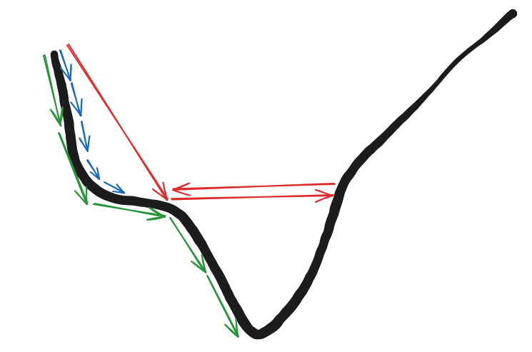
The diagram illustrates the impact of different learning rates on Gradient Descent’s convergence behavior. The Black curve represents a loss function, where the goal is to minimize the loss by moving towards the lowest point. The arrows indicate different learning rates and their corresponding descent paths.
– Red Arrows (Large Learning Rate) :
The step size is too large, causing the updates to overshoot the minimum.
It results in bouncing back and forth, and in extreme cases, the loss may never converge!!
Pros: Moves quickly but only if it stabilizes.
Cons: High risk of diverging, making training unsuccessful.
– Blue Arrows (Small Learning Rate) :
The step size is small, leading to slow but steady convergence.
It might take a long time to reach the minimum, but it avoids overshooting.
Pros: More stable, ensures convergence.
Cons: Computationally expensive due to many small updates.
– Green Arrows (Optimal Learning Rate) :
The step size is just right, allowing the model to reach the minimum efficiently.
It balances speed and stability, reducing training time while ensuring convergence.
This is the ideal learning rate for efficient training.
Now, you might be thinking: I’d rather just give it more time——after all, a smaller learning rate can effectively find the lowest loss.
But what if the loss function looks like this?
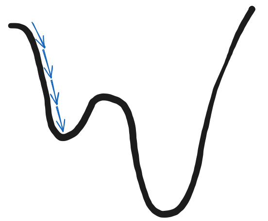
In this case, we need to introduce a new method: Momentum
Momentum in Gradient Descent
What is Momentum?
Momentum is a modification of Gradient Descent that smooths the optimization process, preventing it from getting stuck in local minima.
Think of it like a rolling ball——it doesn’t just consider the current gradient but also accumulates past gradients to make the descent smoother and speed up convergence.
Momentum Formula
$$v:=βv−α∇J(θ)$$
$$θ:=θ+v$$
Where:
v → Velocity (accumulated gradient direction)
β → Momentum coefficient (typically between 0.9 and 0.99)
Key Effects of Momentum on Training Speed
Momentum + Learning → Helps Gradient Descent converge faster and reduces oscillations.
Without Momentum → The optimizer might slow down in flat regions or get stuck in local minima.
RMSProp (Root Mean Square Propagation)
Understanding RMSProp
RMSProp automatically adjust the learning rate based on gradient magnitudes for different parameters. This helps prevent vanishing gradients (where gradients become extremely small, causing training to stall).
Vanishing Gradient: occurs when the gradients in a neural network become extremely small during backpropagation, causing earlier layers to update very slowly or not at all, which hinders effective learning.
Formula
$$E[g^2]_t = \beta E[g^2]_{t-1} + (1 – \beta) g^2$$
$$\theta := \theta – \frac{\alpha}{\sqrt{E[g^2]_t + \epsilon}} \nabla J(\theta)$$
Where:
\(E[g^2]_t\) → Exponentially weighted moving average of squared gradients
ϵ → Small constant to prevent division by zero
Pros: Adapts learning rates for different gradients → More stable learning
Cons: May suppress gradients too much → Learning rate can become too small
Adam (Adaptive Moment Estimation)
What is Adam Optimizer?
Adam combines Momentum + RMSProp, incorporating the best of both methods.
– Momentum → Speeds up convergence by considering past gradients.
– RMSProp → Adapts learning rates for different parameters.
This makes Adam one of the most widely used optimizers in deep learning.
Adam Formula
$$m_t = \beta_1 m_{t-1} + (1 – \beta_1) g_t$$
$$v_t = \beta_2 v_{t-1} + (1 – \beta_2) g_t^2$$
$$\theta := \theta – \frac{\alpha}{\sqrt{v_t} + \epsilon} m_t$$
Where:
\(m_t\) → First moment estimate (similar to Momentum)
\(v_t\) → Second moment estimate (similar to RMSProp)
\(theta\) → Represents the parameters of the model (updated in each step using the corrected first and second moments)
Pros: Automatically adjusts learning rates → Works well in most cases
Cons: May be unstable during convergence
General Recommendation
If unsure which optimizer to use, Adam is often the safest choice due to its adaptability.
Implementation in PyTorch
import torch
import torch.nn as nn
import torch.optim as optim
import matplotlib.pyplot as plt
import numpy as np

# Set random seeds for reproducibility
torch.manual_seed(42)
np.random.seed(42)

# Generate synthetic data (regression): y = x^3 + noise
N = 200
x = np.linspace(-1, 1, N).reshape(-1, 1)
y = x**3 + 0.1 * np.random.randn(N, 1)

# Convert numpy arrays to torch tensors
x_tensor = torch.tensor(x, dtype=torch.float32)
y_tensor = torch.tensor(y, dtype=torch.float32)

# Define a simple feedforward neural network model
def get_model():
    model = nn.Sequential(
        nn.Linear(1, 10),
        nn.ReLU(),
        nn.Linear(10, 1)
    )
    return model

# Training function: runs the training loop and records loss history
def train_model(model, optimizer, x, y, epochs=200):
    criterion = nn.MSELoss()
    loss_history = []
    for epoch in range(epochs):
        optimizer.zero_grad()
        outputs = model(x)
        loss = criterion(outputs, y)
        loss.backward()
        optimizer.step()
        loss_history.append(loss.item())
    return loss_history

# Prepare a dictionary of optimizers to compare
optimizer_configs = {
    "SGD": lambda model: optim.SGD(model.parameters(), lr=0.01),
    "SGD_momentum": lambda model: optim.SGD(model.parameters(), lr=0.01, momentum=0.9),
    "RMSprop": lambda model: optim.RMSprop(model.parameters(), lr=0.01),
    "Adam": lambda model: optim.Adam(model.parameters(), lr=0.01)
}

# Save an initial state dict so that all models start from the same weights
base_model = get_model()
initial_state = base_model.state_dict()

# Dictionary to store the loss history for each optimizer
results = {}

# Train a new model with each optimizer using the same initialization
for opt_name, opt_func in optimizer_configs.items():
    model = get_model()
    model.load_state_dict(initial_state)  # Ensure identical starting weights
    optimizer = opt_func(model)
    loss_history = train_model(model, optimizer, x_tensor, y_tensor, epochs=200)
    results[opt_name] = loss_history

# Plot the loss curves for each optimizer
plt.figure(figsize=(8, 6))
for opt_name, loss_history in results.items():
    plt.plot(loss_history, label=opt_name)
plt.xlabel('Epoch')
plt.ylabel('Mean Squared Error (MSE) Loss')
plt.title('Comparison of Optimization Algorithms')
plt.legend()
plt.grid(True)
plt.show()
Result of different Algorithms
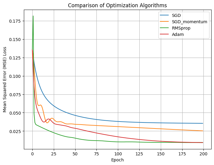
Understanding the Training Process and Results
This chart compares 4 different optimization algorithms (SGD, SGD with Momentum, RMSProp and Adam) on the same neural network model with and identical learning rate. Here are the key takeaways:
1.SGD (Stochastic Gradient Descent): The slowest to converge and prone to getting stuck in local minima. This is because SGD updates weights directly along the gradient descent direction without additional mechanisms to accelerate or smooth the optimization process.
2.SGD with momentum: Introduces a “momentum” parameter that accumulates past gradient directions, making updates similar to a rolling ball, reducing oscillations, and accelerating convergence. As seen in the graph, it descends faster and more smoothly compared to pure SGD.
3.RMSProp: An advanced optimizer that adjusts the learning rate using a moving average of squared gradients, allowing more flexibility in adapting to different gradient scales. RMSProp results in a smoother reduction in MSE Loss and converges quickly.
4.Adam: Combines the benefits of both Momentum and RMSProp, using first and second moment estimates to adapt the learning rate dynamically. Adam is often the go-to choice in deep learning applications due to its fast convergence and insensitivity to hyper parameters. The graph shows that Adam decreases loss quickly and reaches a low MSE Loss.
Why Didn’t We Focus on Standard SGD?
Although SGD is included in this experiment, its performance is noticeably inferior to the other methods-it converges much slower and results in a higher MSE Loss. In practical deep learning applications, pure SGD is rarely the best choice, especially for complex models and non-convex optimization problems, pure SGD is rarely the best choice, especially for complex models and non-convex optimization problems. This is why RMSProp and Adam are more commonly used.
Reference:Prof. Hung-Yi Lee’s Youtube channel